3 Turing patterns, repetitive patterning
A foundational work in Theoretical Biology is Alan Turing’s paper “The Chemical Basis of Morphogenesis” (Turing (1990)). In this work, Turing mathematically demonstrates a plausible mechanism whereby a reaction-diffusion system can lead to the formation of a spatially-patterned solution in steady state. Mathematically and conceptually, Turing’s key innovation was considering diffusion-driven instability. That is: A non-patterned steady state solution becomes unstable in the presence of diffusion, leading to the formation of a spatially patterned state.
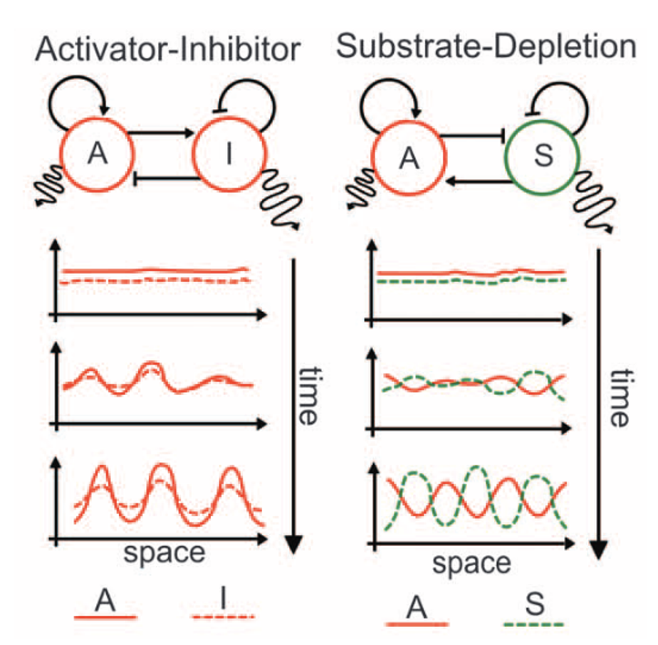
Turing-type patterns emerge when a system exhibits short-ranged activation and long-ranged inhibition. The most well-known realization of a Turing reaction-diffusion system is the combination of a slow-diffusing activator and fast-diffusing inhibitor. Many more examples exist which can be reduced to a mathematically equivalent form. In this practical, we will explore a 3-component Turing system developed by Raspopovic and coauthors to explain the patterning of fingers on the paws of mice (Raspopovic et al. (2014)).
In this practical you will work with a total of 6 different python codes. Please note that each code simply differs by an extension or modification from the previous code, so that in the end you will have a long script that performs all the steps in one go.
3.1 Equivalence of Turing models
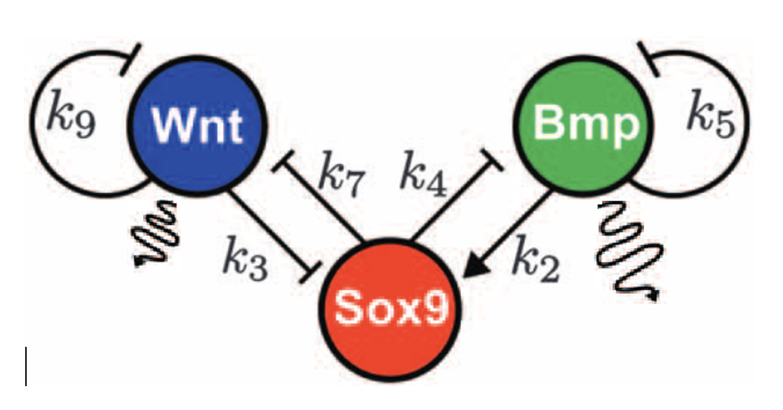
The model proposed by Raspopovic et al. for generating Turing patterns underlying limb bone modeling consists of 3 instead of 2 interacting variables. We will refer to this model as “BSW” model, as it represents interactions between Bmp, Sox9, and Wnt.
Exercise 3.1 (Conceptual thinking) Study the schemes below. The arrows represent activating or inhibiting interactions, while the wavy lines represent diffusion of components. Simplify this 3-variable model scheme into a 2 variable model scheme (just by drawing the interactions, no need to write equations) and explain how it satisfies the Turing conditions discussed in the lecture. Remember that for Turing patterns we need an activator an inhibitor.
In a 2 variable system the activator needs to be a single autoactivating molecule. When we have more variables, the positive feedback can be achieved differently (indirectly). So think which two variables would be logical to combine into one to get a 2 variable model..
3.2 Patterning in a fixed domain size
The code in the script 01__digits_squarehomogeneoustissue.py simulates the model in a 2D square tissue of constant size. This setup can be considered as a small region of a large Petri dish in which mesenchymal cells have been plated with the correct chemicals to undergo bone formation (Supplementary Figure S3 in the paper).
Exercise 3.2 (Biology) Play with parameters \(k4\) (Sox9 effect on BMP), \(k7\) (Sox9 effect on Wnt), and how much Bmp diffusion is faster than that of Wnt. Change one parameter at a time and realise that changing in one direction is sufficient; change in the other direction can be expected to have the opposite effect.
What effects on pattern wavelength do you find?
Note: Make sure to use only small changes for \(k4\) and \(k7\), if things start oscillating wildly or go blank you are watching numerical errors rather than real outcomes. When increasing Bmp diffusion you may need to reduce the time step for integration \(dt\).
3.3 Patterning in a growing domain size
Besides parameter values, the pattern that emerges from a Turing system is also strongly influenced by initial conditions and the size and shape of the domain where reactions and diffusion happen.
In the script 02__digits_growingsquare_PD.py we added tissue growth in the proximo-distal (body to limb) direction. Growth is controlled by a growth rate vi.
Exercise 3.3 (Biology)
- Study the code to understand what it does.
- Increase the horizontal growth rate
viin small increments (try: 0.01, 0.05, 0.1, 0.2, 0.5) and study what happens to the pattern. Explain why you think this happens.
Note: Increase the totaltime parameter to 5000 when using growth rate of 0.01.
3.4 Patterning along two growth axes
In reality, the limb bud grows in both the proximo-distal and anterior-posterior direction. In the script 03__digits_growingsquare.py this is implemented with growth rates vi for proximo-distal growth and vj for anterior-posterior growth.
Exercise 3.4 (Biology) Play with the relative size of these growth rates and study what happens. Compare the order of appearance of stripes to the experimental data in the paper (see Figure 3F in the Raspopovic paper Raspopovic et al. (2014)).
3.5 Making a virtual tissue grow
Think about how tissue growth is implemented in the script 03__digits_growingsquare.py.
Exercise 3.5 (Algorithmic and conceptual thinking) What is the default value of the newly added tissue when it grows? Is the concentration elsewhere in the tissue changed?
Do you think this approach is reasonable to model biological growth of a tissue? Explain why/why not.
Hint: Think about it from the perspective of a growing cell containing a number of molecules “X”.
If the cell increases in volume and does not produce/degrade X, what happens to the concentration of X?
What would be the concentration of X in the two daughter cells if the cell divides?
How would the situation change if X is constantly produced and degraded?
In the paper, @Raspopovic et al. (2014) create a “tissue growth map” (see Figure 3A), which they use to map concentration values from one timepoint to the next using interpolation-based transformations.
Inspired by this approach, the script 04__digits_growingsquare.py implements a different growth function that uses bilinear interpolation to expand the tissue. Play around with the growth rate parameters and compare the results to what you found earlier. Do the patterns differ? If yes, how do they differ?
Hint: Try the supplementary script supp_g__bilinear_interpolation.py to understand how interpolation-based growth works.
For master students: yet another way of implementing tissue growth would be to take cell division and inheritance of maternal state by the two daughter cells literal and implement this by new boundary cells copying the state of their direct neighbors. Implement this alternative growth and see how this affects your results.
3.6 Spatial modulation of parameters k4 and k7
Let us now ignore growth and its role on orienting stripes for a while and explore once again the influence of parameters on the patterns. In reality, digits are patterned further apart at the distal end than at the proximal end, where they need to converge on a hand and wrist. This implies that the wavelength of the Turing pattern should not be constant. In a previous question you probably found that the k7 and k4 parameters impact the wavelength of the Turing pattern. The authors speculate that the FGF and Hox gene gradients observed in the limb bud exert an effect on the Sox9-BMP-Wnt patterning module through these parameters.
Exercise 3.6 (Biology) The script 05__digits_squarek4k7gradient.py allows you to implement exponential gradients of k4 and k7 across the tissue. You can set the minimum and maximum values, axis (x=horizontal, y=vertical) and direction (0=decreasing, 1=increasing). Look in the supplement of the Raspopovic paper, page 48 Fig 2C (Raspopovic et al. (2014)), left for the estimated change of k4 and k7 across the tissue and try to reproduce (not exactly but similarly) Figure 2C, right side, by playing with the parameters affecting the k4 and k7 gradients. Describe along which axis, in which direction and to what extent k4 and k7 are changing. Estimate the change in Turing pattern wavelength this results in.
3.7 Hoxd13 and FGF
As mentioned above, the biological factors thought to underly the variation in the k4 and k7 parameters are Hoxd13 and FGF. Hoxd13 is highly expressed in the distal domain of the paddle and not expressed elsewhere, and this expression domain is growing as the paddle grows. FGF is expressed from the distal edge of the paddle and spreads through diffusion. For an illustration see Fig S8A of the supplement of the Raspopovic paper (page 10 Raspopovic et al. (2014)). Experimental data furthermore suggest that Hoxd13 and FGF together affect k4 and k7, which the authors decided to model using the following equations:
\[ k4^* = k4 - k_{HF_{bmp}} * fgf(i,j) * hox(i,j) \]
\[ k7^* = k7 + k_{HF_{wnt}} * fgf(i,j) * hox(i,j) \]
Exercise 3.7 (Algorithmic and biological thinking) The script 06__digits_squarehoxdfgf.py implements how k4 and k7 are a function of local FGF and Hox values, but does not yet include Hox and FGF spatial patterns and how these develop over time. Adjust the code to incorporate the observed Hoxd13 and FGF patterns and study how the digit patterns compare to what you found under question 7. Note that arrays for hox and fgf are included, and decay and diffusion values for fgf are provided already in the code. Also note that hox and fgf each have a maximum value of 1.
3.8 Shape makes the tissue
Having studied the effects of growth and genetic factors modulating the Turing pattern now it is time for the final step. So far, we’ve approximated the limb bud very crudely with a rectangle. As you probably noticed in your parameter exploration, the tissue boundary can bias stripe orientation. Therefore it is interesting to study the interplay between the shape of the “paddle” or limb bud in which the digits develop and how it grows with the temporal development of the hox and fgf patterns. In the script 07__digits_growingpaddle.py we implemented two different tissue geometries: An ellipse and a “paddle” that imitates the shape of the limb bud. Note that to implement Hox and FGF domains on a complex growing shape, quite a bit of complex code involving masks describing the tissue domain and angles to control the Hox and FGF domains was needed. At first, we are going to ignore these technical details.
Exercise 3.8 (Biology) Switching between geometries is easily done by changing the value of the parameter geometry on line 78 of the script. Start with the “ellipse” geometry. What do you observe with regards to the FGF gradient? What consequences does this have? Why would this be “a smart thing to do”?
Play around with vi/vj and Lx0 to investigate the effect of ellipse shape and development over time on the number, shape and robustness of digits that form.
Now switch to the paddle geometry. Observe the patterns that emerge and compare these to the simulated and experimentally observed patterns in Figure 3E and 3F of the Raspopovic article (Raspopovic et al. (2014)). According to you what does and what doesn’t the model explain well?
To implement non-square geometries, the script uses “masks”. Study how these masks are created in the functions create_ellipse_mask and create_tissue_mask.
Hint: Try the supplementary script supp_i__geometries.py.
Note: For computational convenience, we use the “Class” data structure to implement common functions shared by the masks. This is a somewhat more advanced programming concept, so it’s ok if you don’t understand what it does yet. For the extra curious and motivated, feel free to check out the supplementary script supp_i__class_data_structure.py.
3.9 Master students exercise
Exercise 3.9 (Poly and oligodactyly) Above we played with ellipse size and growth rates, however in addition to mutations affecting tissue size and growth, also mutations in genes affecting the Hox and FGF morphogens may occur. Play with parameters that determine Hox and FGF expression zones on the paddle geometry. Which parameter changes lead to the formation of supernumerary fingers (polydactyly)? Which parameters lead to too few fingers (oligodactyly)?
Hint: The following supplementary scripts will be helpful to understand how the FGF and Hox domains were coded:
supp_i__ellipse_slice.pyvisualizes the usefulness of masks based on the example of selecting a slice of an ellipse;supp_i__smooth_function.pyvisualizes the functionsmooth_function();supp_i__morphological_operations.pyvisualizes morphological operations (binary dilate/erode and Gaussian blur) which are used for mask operations, calculating the Laplacian on the irregular domain, and to select pixels to generate the FGF and Hox pattern;supp_i__maskDifference.pyvisualizes the difference of masks, which is how the functionsingle_step_growth()checks if the tissue domain is growing or shrinking.