6 Cell sorting by differential adhesion

6.1 Morphogenesis

Morphogenesis is the culmination of gene expression, biochemical signaling, and biophysical forces at the cell and tissue levels. These processes are complex and not completely understood, so we don’t yet have a “perfect” model of how we should simulate morphogenesis. For this reason, several research groups independently developed simulation approaches that fit their needs. In this practical, you will get acquainted with one such approach, the cellular Potts model.

6.2 Biological background

Classical experiments in the 1950s dissociated animal embryonic tissues and recombined them in vitro to try to understand the principles of self-organization. Instead of staying mixed, each cell type sorts out into its own region, resembling the organization in the embryo.

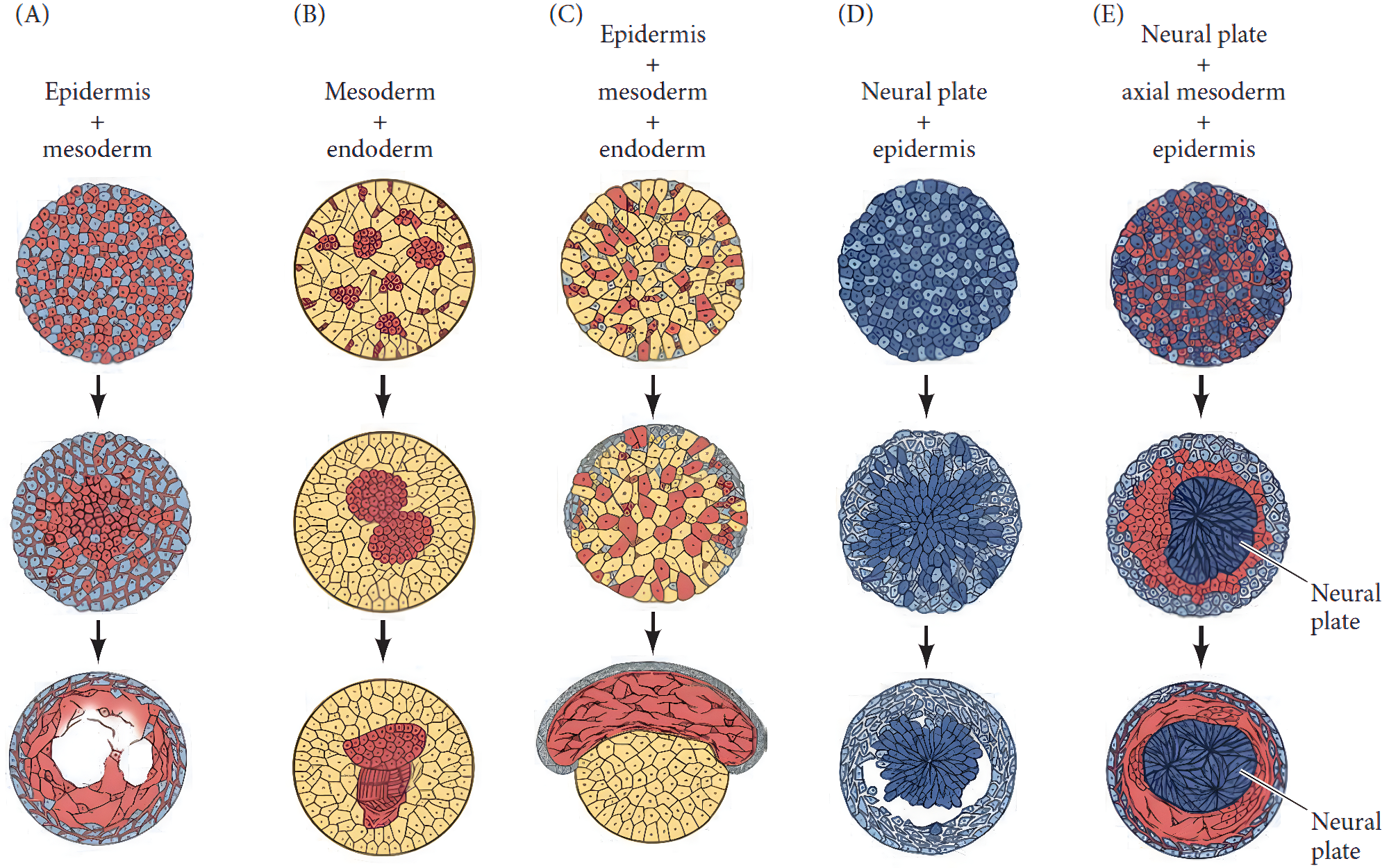
Sorting of aggregates of embryonic cells, based on experiments by Townes and Holftreter in 1955. Image adapted from Gilbert “Developmental Biology” 11th edition.

According to the “differential adhesion hypothesis”, unlike expression levels of cell-cell adhesion molecules is the mechanistic driver of cell sorting. Biophysically, cells form aggregates that minimize the contact energy at interfaces, rearranging into the most thermodynamically stable pattern. In 1992, the cellular Potts model was developed to test this hypothesis using simulations (Graner and Glazier (1992)).

6.3 The cellular Potts / Glazier-Graner-Hogeweg model

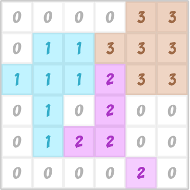
The cellular Potts Model (CPM), also known as Glazier-Graner-Hogeweg (GGH) model after its major developers and popularizers, simulates stochastic dynamics of cell shapes on a grid (=a lattice). The model has its historical roots in physical models of magnetization of metals and formation of foam bubbles, so some of the terminology harkens back to that. Each grid site on the lattice has a spin value σ (Greek small letter sigma), usually an integer number. A biological cell is represented by all lattice sites with equal value σ.

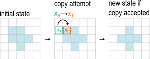
Example of a σ field with four unique integer values. The value 0 is reserved for the medium, while the non-zero values represent three cells.

Cell shapes change by elementary changes called copy attempts, where one site of the lattice (the source site x_S) attempts to copy its σ value to a neighboring lattice site (the target site x_T). Copy attempts can succeed (be accepted) or fail (be rejected).

Every copy attempt affects a pair of neighboring lattice sites.

Choosing and accepting copy attempts occurs via a stochastic Monte Carlo method. More specifically, a modified Metropolis-Hastings algorithm, which is an algorithm that minimizes an energy function H calculated based on the lattice configuration. The probability that a copy attempt is accepted P(accept) depends on the change in energy ΔH between the configuration before and after a copy attempt:

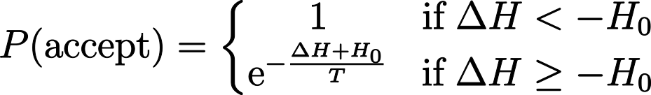
In the above equation, T is a parameter that determines how likely it is that an unfavorable copy attempt that increases the energy is accepted, while H₀ is a parameter representing the yield, that is, how easily the cell membrane changes shape (often, this parameter is set to H₀ = 0). What this equation says is: Configurational changes that lower the energy below at least H₀ are always accepted (probability of 1), while configurational changes that increase the energy are accepted with a probability that decreases exponentially with the energy cost. In a biological sense, cells consume energy from ATP to create configurations that are physically unfavorable (ΔH ≥ -H₀). Therefore, the parameter T can be interpreted as intrinsic cell activity.

6.4 Exercises

Exercise 6.1 (Algorithmic thinking - Anatomy of a cellular Potts model) A minimal cellular Potts model simulation of cell sorting contains the following ingredients:

definition of the “sigma field”
definition of the “tau field”
the initial condition of sigma and tau fields
the neighborhood of a grid site
a Monte Carlo stepping procedure
definition and calculation of the energy function H

Study the code provided in the script 01_cpm.py. Then, answer the following questions:

Which functions in the script correspond to the above ingredients?
What is the default initial condition?
What is the default neighborhood?
Run the script and observe the plots that appear. Explain in your own words what is the sigma field and what is the tau field. Do you understand why two different fields are needed?

Exercise 6.2 (Conceptual thinking - Interpreting the Hamiltonian energy function) The Hamiltonian energy function H is at the heart of a CPM/GGH simulation. H reflects our assumptions about the system and how forces affect the cell (the derivative of energy with respect to position is force).

In the script 01_cpm.py, the following Hamiltonian is used.

where J is a symmetric matrix of interfacial energies for all cell type pairs τ (small Greek letter tau), A(σ) is the area sum of lattice sites belonging to spin σ, A_0,τ(σ) is the “target” area of the corresponding cell type τ, and λ_A(τ(σ)) is a weighting factor that scales the importance of this term (also known as Lagrange multiplier). Each term represents a constraint.

Perhaps a more intuitive way to understand the terms is the following pseudo-code:

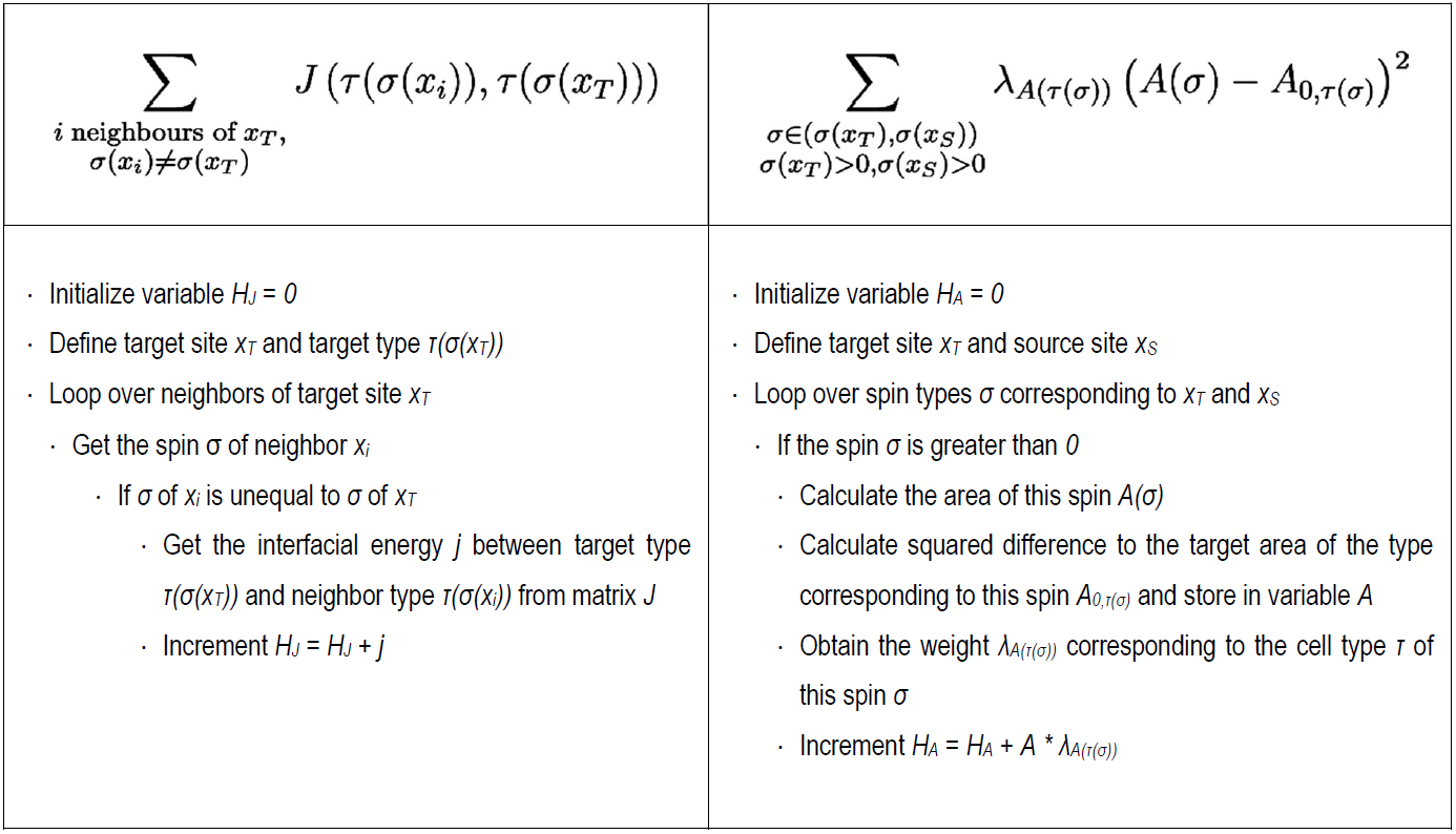
Compare the pseudo-code to the implementation in the script. Then answer the following questions:

What are the biological processes modeled with this specific energy function?
Take a closer look at the summation terms. Over which domain is the first sum calculated? What about the second summation term?

Exercise 6.3 (Conceptual thinking - How parameters affect the Hamiltonian energy function) The modified Metropolis algorithm used in the Monte Carlo stepping procedure ensures that over time, on average, the sum of the energy of the entire sigma field will reach a minimum. However, the different Hamiltonian terms may work “against” each other: minimizing one term may lead to maximizing the value of the other term.

Let’s vary the parameters that affect the Hamiltonian terms to get an intuition for how they work. In the following, you may want to take screenshots of the final simulation state to put in your notes, so that it’s easier to compare the outputs.

Change the default neighborhood to “8” and run the simulation again. What happens?
Keep the neighborhood at “8”, and increase the parameter for “volume_weight” from [1, 1] to [2, 1]. Then, run the simulation again. What happens?
Change the initialization mode (“init_mode”) from “random_pixel” to “square_grid”, and reset the parameter “volume_weight” to [1, 1]. What happens now if you simulate?
Explain why these settings and parameters that you just changed affect the simulation outcome.

Exercise 6.4 (Algorithmic thinking - The Monte Carlo update algorithm) In addition to showing a visualization of the σ and τ fields, the script 01_cpm.py also prints some information to the terminal.

Reset all parameters to their default values, then, based on the printed information, answer the following questions:

How many copy attempts are made in total in one Monte Carlo Step?
How many of these copy attempts are accepted on average?
- Calculate the average for 5 Monte Carlo Steps across 3 simulation runs.
How many seconds does it take to run one simulation?
- Calculate the average run time for 3 runs.

The script 01_cpm.py uses the traditional update algorithm. In this algorithm, every copy attempt picks a target site randomly among all lattice sites, then subsequently picks a source site randomly among the neighbors of the target site. This leads to many invalid lattice pairs that are always rejected. The edge list algorithm is a clever way of speeding up this procedure by restricting copy attempts only to those interfaces where there is a possibility of acceptance.

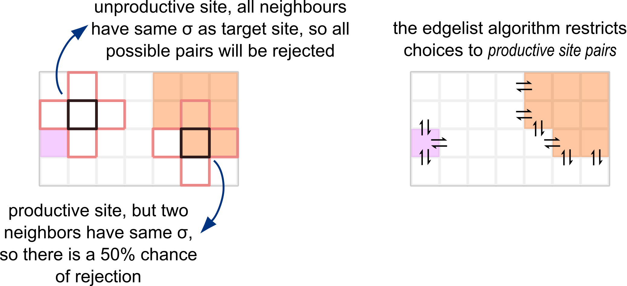
Since a copy attempt affects a pair of neighboring lattice sites, we can keep track of valid pairs (productive site pairs). These can be represented by an edge, i.e. an arrow pointing from one site to the other. Edges have a directionality, so two neighboring sites are always joined by two edges with opposing direction.

The script 02_cpm_edgelist.py implements the edge list algorithm. It’s quite complicated, so don’t worry about understanding all the technical details. Using this script, answer the above questions again and compare to the results you got with the traditional update algorithm.

Explain: Why does the edgelist algorithm reduce computation time? In which situations would you expect the difference in computation time between algorithms to be large?

Exercise 6.5 (Biology - Expanding the Hamiltonian) Suppose you want to add more mechanisms for cell shape changes to the model. This would involve the following steps:

Coming up with a hypothesis on how forces act on the cell shape.
Deriving a mathematical function that establishes the energy balance.
Add an additional function to the code that calculates the energy based on the cell configuration.
Call this function in the code that calculates the energy differential.

Let’s walk through these steps together to create a perimeter constraint.

Animal cells possess a contractile actomyosin cortex connected to the cell membrane via actin-membrane linker proteins. Cortex contraction is regulated to maintain homeostasis of the membrane tension. Simply put, if the cell membrane gets “floppy”, the cortex contracts to pull the membrane in. Vice-versa, if the membrane is too tense, cortex contractility is reduced to allow the membrane to relax. We thus could advance the hypothesis that forces from the actin cortex strive to maintain a constant cell surface area.
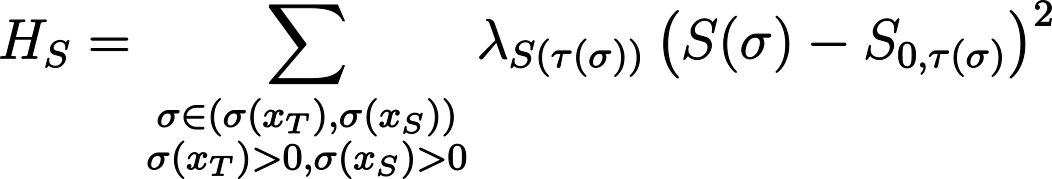
We want cell surface area to reach a target homeostatic value S₀. Let’s call the actual cell surface area S. We need a function that has a minimum where S₀ = S and increases if S is larger or smaller than S₀. A simple function that does the trick is the parabola (S- S₀)². We may also want to tune how much this term influences the entire Hamiltonian, so we introduce the weight factor λ_S. We also consider that both S₀ and λ_S may depend on cell type τ.

Thus, we write:

For the implementation of steps 3 and 4, consult the script 03_cpm_perimeter.py.
Study the new additions to the script (search for the string: ### NEW ### to find them quickly), then run the simulation. Vary the parameters to gain an intuition of how this new Hamiltonian term affects the simulation outcome.
You may have noticed the simulation is running more slowly than before. Review the new code additions again. Can you identify any potential reasons for this decrease in computation speed?

Exercise 6.6 (Biology - Imposing cell connectivity) In the previous simulations you ran, you may have noticed that cells sometimes break up into disjointed fragments. There are two alternative ways to prevent this: 1. Add a new Hamiltonian term that penalizes copy attempts that would break up the cell. 2. Modify the update algorithm to always reject copies that would break cells apart.

Script 04_cpm_connectivity.py implements the second option using a flood fill algorithm to count the number of contiguous pixels of the non-medium target cell supposing that a copy succeeded.

Try out the simulation!

Can you think of advantages and disadvantages to using the first or second option?
Once again, the simulation is running more slowly than before. What parts of the new code do you suspect may be causing the slowdown?

Exercise 6.7 (Biology - Exploring differential adhesion and cell sorting) Now let’s explore how changing adhesion affinities leads to different sorted cell configurations. To do that, you will need to run simulations for a longer time. To speed up computations, you will be using an optimized package (many scripts working together), which is contained in the folder “cellularPotts”. To make visualizations super-fast, this package uses the PyQt5 module, which should be installed by default with your Anaconda distribution.

Note: If for some reason you cannot get PyQt5 to work, there is an alternative package that uses matplotlib “cellularPotts_MPL”. However, this runs much slower.

To launch the simulation, run the main.py file in the cellularPotts folder. You can change the parameters by adjusting values in the parameters.py file.

Adjust the values of the adhesion table for the two cell types:

Set equal adhesion affinities for all cell-cell interactions. Leave affinity to the medium at a low value.
Set the adhesion affinity of cell type 1 to itself to a larger value.
Set the affinities such that cell-medium interactions are more favorable than any cell-cell interactions.
Explore how other parameters such as volume and surface constraints affect the cell sorting simulations.

(Master students) Add a third cell type to the simulation by editing the parameter.py file. Can you get a sorted configuration where cell type 1 envelops cell type 2, which itself envelops cell type 3?

References

[1] Gilbert and Barresi (2016) (https://utrechtuniversity.on.worldcat.org/oclc/1035852599)

[2] Graner and Glazier (1992) (https://doi.org/10.1103/PhysRevLett.69.2013)