11 Modeling Thermomorphogenesis in Plants
Plants respond to temperature not only through metabolic changes but also by adjusting their morphology. A well known response of plants to increased ambiant temperature is the lifiting of their leaves (hyponasty) and increasing their petiole (stalk between leaf and stem) length to lower the internal leaf temperature. It is thought that this may help plants cope with heat, but it’s not always clear whether and if so how this actually improves growth. In this practical, we will use and extend a small ODE model of carbon (C) and leaf area (LA) dynamics and explore how temperature and thermomorphogenic responses affect growth. You’ll simulate different temperature conditions and analyze how traits like leaf angle and size affect photosynthesis and carbon respiration rate, and how this affects overall plant growth. Later, you will investigate the adaptive value of this response, as this is still an open question.
11.1 The model
In code 00_Environment_and_development.py we start with a simple two ODE model where leaf area (\(L\)) grows with rate \(G\), which depends on carbon concentration (\(C_c\)) and leaf area. Carbon (\(C\)) is produced by photosynthesis (\(P\)) dependent on leaf area, leaf angle (\(\alpha\)), and temperature (\(T\)). Carbon is consumed by growth and respiration (\(R\)), dependent on temperature and leaf area again:
\(\frac{dC}{dt}=P(L,T,\alpha)-R(L,T)-G(C_c,L)\)
\(\frac{dL}{dt}=G(C_c,L)\)
Photosynthesis
Photosynthesis is a complex process that can be modeled in many different ways with varying complexity. Here, in the function Photosynthesis_per_m2() we included a semi-detailed photosynthesis model based on the assumption that the protein RubisCo is the limiting step in photosynthesis. This model has 6 parameters and 2 environmental variables, of which all parameters are temperature sensitive. This temperature sensitivity is based on the Arrhenius equation, which describes the temperature dependency of chemical reaction rates.
Maintenance Respiration
Maintenance respiration is a term used in biological systems to describe all energy/carbon consuming processes that a plant must do to survive. Similar to photosynthesis, the rates of these reactions increase with temperature, and as such, carbon costs greatly increase. We model this in the function Respiration_per_m2() using the Q10 equation, that describes how much a rate increases for 10 degrees of temperature increase.
11.2 Exercises
Exercise 11.1 (Algorithmic thinking and Biology - Temperature Effects on Photosynthesis, Respiration and Growth) Let us first investigate how photosynthesis and respiration depend on temperature.
Plot photosynthesis and respiration rate as a function of temperature, using the functions defined above. Explain: What happens to net carbon gain at high temperature? Why is high temperature problematic for growth in this model?
Run the code and study the output for leaf area and carbon. Why does leaf area increase exponentially while carbon levels saturate? What carbon level are you actually plotting?
Now run simulations of the ODE model for low (15°C), medium (25°C), and high (35°C)
temperatures. Which plant performs best? Which plant worst? Why is this?
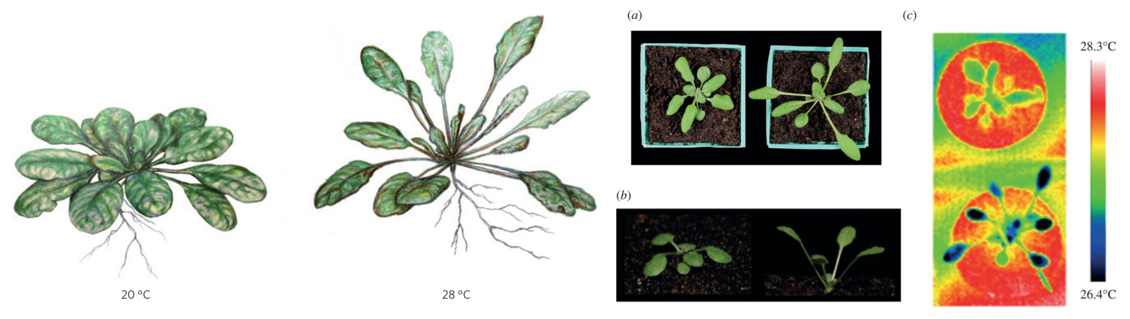
Exercise 11.2 (Mathematical & Biological thinking - Hyponasty – Leaf angle increase) Until now we have investigated the effect of temperature on plants that do not respond to their environment, but plants do respond to their surroundings. Plants display a variety of responses to elevated temperature, and one of these is so-called leaf hyponasty in which leaves are positioned in a more upward orientation that is often accompanied by longer leaf stems (petioles) and smaller leaves (blades). Let us extend the model to first simply include the orientation aspect of this hyponastic response to high temperature.
- The photosynthesis function already includes a term for ‘effective leaf area (LA_eff)’, but the function does currently return the total leaf area. Rewrite this function to return effective leaf area as a function of leaf elevation angle, assuming that light comes from above. Plot the effective leaf area as a function of angle. How does hyponasty affect photosynthesis? What other factors could affect effective leaf area?
- Now investigate the effect of the increased leaf angle on plant growth. Compare medium (25°C) and high temperature (35°C) for normal (20°) and increased (40°) angle.
Exercise 11.3 (Biology - Hyponasty– Cooling Benefit) Leaf hyponasty is shown to lower leaf temperature with a few degrees by improving heat dissipation and decreasing the area in which direct sunlight hits the leaves.
Investigate the effect of the leaf cooling. How much cooling is needed for hyponasty to have a net positive effect? Simply assume a certain cooling effect and hence apply a lower temperature than the environmental one.
Hyponasty is shown to lower leaf temperature by only 1-2°C (see the left panel in Figure 1), what is the effect of this amount of cooling on plant growth? Would you argue that this hyponastic response is adaptive in the current model (i.e. assuming no other factors play a role)?
Reanalyze the curves describing how photosynthesis rate depends on temperature and how effective leaf area depends on angle and explain your earlier results.
Exercise 11.4 (Biology -Is hyponasty adaptive?) The cooling down of the leaves through hyponasty is thought to be an important adaptive trait. Interestingly, from the simulations we’ve done so far this adaptive advantage is not very clear. It might therefore very well be that we miss important processes in the current model. In this last question of the practical you will extend the model with additional processes also relevant in plants to see if this may help explain the adaptiveness of hyponasty. This is also an open question in current research, so there is no clear answer and you might actually come up with novel ideas! To help guide your thinking, we have come up with some additional plant processes you can implement and investigate to see how these impact adaptiveness of leaf hyponasty under high temperature. Pick one to work on and investigate if this would render hyponasty more clearly adaptive. If you have extra time, see if you can combine them. If you have other ideas to work on, this is also great! You can use the answer code 03_Environment_and_development_answers.py (at the bottom of this page) as a starting point.
- Hypothesis 1 - Day-Night Rhythm
We found that during the day, while hyponastic cooling brings photosynthesis closer to its optimum temperature and reduces respiration, this is insufficient to overcompensate the costs of reduced effective leaf area. During the night, cooler leaf temperatures still reduce maintenance respiration, while photosynthesis halts and hence reduction of effective leaf area plays no role, suggesting at night time hyponasty has only advantages. To investigate whether this results in a net adaptive effect of leaf hyponasty incorporate the following processes in your model: - Temperature: Simulate the cooling effect of nighttime. - Photosynthesis: Photosynthesis does not occur without sunlight, so simulate the change of light over the day and its effects. - Respiration: Maintenance respiration persists in absence of photosynthesis. - Hyponasty changes: Leaf angles change over the course of a day, reaching a minimum early during the day and being relatively high during the night. - Growth rate: Counterintuitively in plants often most growth happens during the night, when water loss is minimal and hence turgor pressure is high.
Hint: use sine functions to describe the daily rhythms and their relative phases. Make sure that light is really zero at night . As an example you can write things as:
Tvar=max(0,3*T/4+T/4*np.sin(2*np.pi*(t-6)/24))
which says that the actual variable temperature \(Tvar\) is a sine function of the imposed temperature T, has a 24 hour period, is phase shifted 6 hours to have the highest temperature at 12 and not 6 o’ clock during the day. Note that since a sine function has a maximum of 1 and a minimum of -1, the ¾ and ¼ fractions serve to make temperature vary between ½ and 1 of the imposed temperature T. The max function serves to ensure that the overall result can not go below 0.
a1. Analyze how the absence of photosynthesis at night affects carbon balance. Do you think what you see happening is reasonable? How could you repair this?
a2. Examine the impact of nighttime temperatures on maintenance respiration rates.
a3. Explore how changes in leaf angle influence overall plant growth.
a4. Now combine the two
- Hypothesis 2 – Stomata
Stomata play a critical role in regulating gas exchange and water loss in plants. As leaf temperature increases, stomata open to enhance transpiration, which cools the leaf through evaporative cooling. This mechanism is particularly effective in well-watered plants, where increased stomatal opening can significantly reduce leaf temperature up to around a maximum of 9-10°C. However, at very high temperatures, stomata may close to prevent excessive water loss, which can lead to overheating. Additionally, stomatal opening increases while stomatal closing decreases photosynthesis rates by affecting gas exchange efficiency. Thus, incorporating this dependence of stomatal aperture on temperature may enhance the detrimental effects of high temperature, offering more opportunity for leaf cooling effects of hyponasty to matter.
To model this, implement the following changes: - Stomatal opening affects photosynthesis: Include in the photosynthesis function a multiplication factor for stomatal aperture. - Stomatal opening depends on temperatures: Include a function that describes how stomatal aperture first increases with temperature, reaches a maximum at around 25 degrees and then declines for higher temperatures. Aperture should be approximately half the maximum value for temperatures of 10 degrees and 35 degrees. - Stomatal opening increases transpiration: Simulate the cooling effect of transpiration on leaf temperature.
Hint: Now that you have two factors affecting temperature, leaf angle and stomatal aperture, it is a good idea to write a function for leaf temperature in which the combined effect is computed.
Analyze how stomatal opening affects leaf cooling and photosynthesis under moderate temperature conditions. Investigate the trade-offs between cooling benefits and photosynthesis efficiency at very high temperatures. Examine how stomatal closure impacts plant growth and carbon balance under heat stress.
11.3 References
Look at this: hyponasty angle quite high during night, dips early in the day Praat et al. (2024)
Normal and shade avoidance hyponasty is still large in the dark, and dips around dawn for long day conditions: Michaud et al. (2017)
For short day conditions it even peaks during the dark and is lower during day: Oskam et al. (2023) and Dornbusch et al. (2012)
import numpy as np
import matplotlib.pyplot as plt
from scipy.integrate import solve_ivp

"""Parameters"""
Pmax = 1     #Max Photosynthesis rate
R25  = 0.2    #Respiration rate at 25C
Gmax = 0.25  #Max growth rate
K_g  = 2     #Value where growth is at half max.

#Three temperatures to test
T1=15; T2=25;T3=35

""" Functions """
## Calculate Respiration normalized for a reference temperature of 25C
def Respiration_per_m2(T,Q10):
    Resp    = Q10 ** ( (T-25) / 10)
    return Resp

## Calculate Realtive Photosynthesis with a reference temperetaure of 25C
def Photosynthesis_per_m2(T):
    # This function calculates the temperature dependency of photosynthesis parameter values
    def TempDependency(c, dHa,T):
        R = 8.31e-3
        T = T + 273
        return  np.exp(c - dHa/(R*T))

    #This function calculates photosynthesis at temperature T and at 25C and returns A_T/A_25
    ci = 230; O = 210
    VcMax  = 98*TempDependency(26.35,65.33,T)
    VoMax  = 98*TempDependency(22.98,60.11,T)
    Kc     = TempDependency(38.05,79.43,T)
    Ko     = TempDependency(20.30,36.38,T)
    G_Star = TempDependency(19.02,37.83,T)
    R_D    = 1.1*TempDependency(18.72,46.39,T)

    VcMax25  = 98*TempDependency(26.35,65.33,25)
    VoMax25  = 98*TempDependency(22.98,60.11,25)
    Kc25     = TempDependency(38.05,79.43,25)
    Ko25     = TempDependency(20.30,36.38,25)
    G_Star25 = TempDependency(19.02,37.83,25)
    R_D25    = 1.1*TempDependency(18.72,46.39,25)

    A = (1 - G_Star/ci) *( VcMax * ci / (ci + Kc*(1 + O/Ko))) - R_D #Photosynthesis Rate
    A25 = (1 - G_Star25/ci) *( VcMax25 * ci / (ci + Kc25*(1 + O/Ko25))) - R_D25 #Photosynthesis Rate at 25C

    return A/A25

def EffectiveLeafArea(LA,angle):
    """
    Calculate the effective leaf area based on the leaf area and angle.
    """
    return LA

def Photosynthesis(LA, T,angle):

    # Photosynthesis rate depends on leaf Temperature
    TempPhoto = Photosynthesis_per_m2(T)

    #Photosynthesis goes down with increased leaf angle - assuming light comes from the top
    LA_eff = EffectiveLeafArea(LA, angle)

    return Pmax * TempPhoto *  LA_eff

def Respiration(LA,T,Q10):

    TempResp    = R25 * Respiration_per_m2(T, Q10)

    return TempResp *  LA

def Growth(C_conc, LA):
    #LA increase saturates with Carbon concentration in the leaf
    return Gmax* C_conc/(C_conc+K_g) * LA

def ODE_system(t, y, T, angle):
    C, LA = y;    C_conc=C/LA

    dCdt =  Photosynthesis(LA, T,angle) - Respiration(LA,T,2.5) - Growth(C_conc,LA)
    dLAdt = Growth(C_conc,LA)

    return [dCdt, dLAdt]


"""Investigate how photosynthesis (specificity vs. turnover) and respiration (Q10 principle, assume Q10 =2) depend on Temperature - use functions in HelperFunctions.py
Photosynthesis can be normalized to 25C by dividing A over A25 """

T = np.linspace(10,40,100); Q10 = 2
P  = Photosynthesis_per_m2(T)
R  = Respiration_per_m2(T, Q10)

plt.figure()
plt.plot(T, P*100, label='Photosynthesis')
plt.plot(T, R*100, label='Respiration')
plt.ylim(0,250)
plt.legend()

plt.ylabel('Rate (% compared to T=25C)')
plt.xlabel('Temperature (C)')
plt.tight_layout()
plt.show()

"""Run simulations of the ODE model for low (15°C), medium (25°C), and high (35°C) temperatures.
Which plant performs best? Which plant worst? Why is this?"""
# Initial conditions
y0 = [2.5, 2.5]  #Initial LA and C state of the plant

# Time span of the simulation
tend=24; t_eval = np.linspace(0, tend, 100)

T15 = solve_ivp(ODE_system, (0,tend), y0, t_eval=t_eval, args=(T1,25,))
T25 = solve_ivp(ODE_system, (0,tend), y0, t_eval=t_eval, args=(T2,25,))
T35 = solve_ivp(ODE_system, (0,tend), y0, t_eval=t_eval, args=(T3,25,))

# Plot results
fig,(ax1,ax2) = plt.subplots(1,2)
ax1.plot(T15.t, T15.y[1],label='T=15')
ax1.plot(T25.t, T25.y[1],label='T=25')
ax1.plot(T35.t, T35.y[1],label='T=35')
ax1.set_xlabel('Time (-)'); ax1.set_ylabel('Leaf Area')
ax1.legend()
ax1.set_ylim(0,50)

ax2.plot(T15.t, T15.y[0]/T15.y[1],label='T=15')
ax2.plot(T25.t, T25.y[0]/T25.y[1],label='T=25')
ax2.plot(T35.t, T35.y[0]/T35.y[1],label='T=35')
ax2.set_xlabel('Time (-)'); ax2.set_ylabel('Carbon')
ax2.legend()
plt.tight_layout()

plt.savefig('Growth_Q1.png')

plt.show()import numpy as np
import matplotlib.pyplot as plt
from scipy.integrate import solve_ivp
"""Parameters"""
Pmax = 1 #Max Photosynthesis rate
R25 = 0.2 #Respiration rate at 25C
Gmax = 0.25 #Max growth rate
K_g = 2 #Value where growth is at half max.
#Three temperatures to test
T1=15; T2=25;T3=35
## Calculate Respiration (1/m2/s) normalized for a reference temperature of 25C
def Respiration_per_m2(T,Q10):
Resp = Q10 ** ( (T-25) / 10)
return Resp
## Calculate Realtive Photosynthesis with a reference temperetaure of 25C
def Photosynthesis_per_m2(T):
# This function calculates the temperature dependency of photosynthesis parameter values
def TempDependency(c, dHa,T):
R = 8.31e-3
T = T + 273
return np.exp(c - dHa/(R*T))
#This function calculates photosynthesis at temperature T and at 25C and returns A_T/A_25
ci = 230; O = 210
VcMax = 98*TempDependency(26.35,65.33,T)
VoMax = 98*TempDependency(22.98,60.11,T)
Kc = TempDependency(38.05,79.43,T)
Ko = TempDependency(20.30,36.38,T)
G_Star = TempDependency(19.02,37.83,T)
R_D = 1.1*TempDependency(18.72,46.39,T)
VcMax25 = 98*TempDependency(26.35,65.33,25)
VoMax25 = 98*TempDependency(22.98,60.11,25)
Kc25 = TempDependency(38.05,79.43,25)
Ko25 = TempDependency(20.30,36.38,25)
G_Star25 = TempDependency(19.02,37.83,25)
R_D25 = 1.1*TempDependency(18.72,46.39,25)
A = (1 - G_Star/ci) *( VcMax * ci / (ci + Kc*(1 + O/Ko))) - R_D #Photosynthesis Rate
A25 = (1 - G_Star25/ci) *( VcMax25 * ci / (ci + Kc25*(1 + O/Ko25))) - R_D25 #Photosynthesis Rate at 25C
return A/A25
def EffectiveLeafArea(LA,angle):
"""
Calculate the effective leaf area based on the leaf area and angle.
"""
return np.cos(np.radians(angle)) *LA
def Photosynthesis(LA, T,angle):
# Photosynthesis rate depends on leaf Temperature
TempPhoto = Photosynthesis_per_m2(T)
#Photosynthesis goes down with increased leaf angle - assuming light comes from the top
LA_eff = EffectiveLeafArea(LA, angle)
#Max Photosynthesis rate
Pmax = 1
return Pmax * TempPhoto * LA_eff
def Respiration(LA,T,Q10):
#Respiration rate at 25C
R25 = 0.2
TempResp = R25 * Respiration_per_m2(T, Q10)
return TempResp * LA
def Growth(C_conc, LA):
#LA increase saturates with Carbon concentration in the leaf
return 0.25 * C_conc/(C_conc+2) * LA
def ODE_system(t, y, T, angle):
C, LA = y; C_conc=C/LA
dCdt = Photosynthesis(LA, T,angle) - Respiration(LA,T,2.5) - Growth(C_conc,LA)
dLAdt = Growth(C_conc,LA)
return [dCdt, dLAdt]
""""
Until now, we have looked at the differences between temperatures for plants that do not respond to their environment
In reality, plants respond to their surroundings. Plants have a so-called thermomorpogenic response, in which it is observed that they lift
their leaves (leaf hyponasty, increased leaf angle) when temperatures are high. This is thought to be a response to prevent overheating of the leaves.
"""
#plot effective leaf area as a function of angle
plt.figure()
angle = np.linspace(0, 90, 100)
plt.plot(angle, EffectiveLeafArea(1,angle))
plt.xlabel('Leaf Angle (Degrees)')
plt.ylabel('Effective Leaf Area')
# Initial conditions
y0 = [2.5, 2.5] #Initial LA and C state of the plant
# Time span of the simulation
tend=24; t_eval = np.linspace(0, tend, 100)
#Two temperatures to test
T2=25;T3=35
#Two angles to test
angle1 = 20; angle2 = 40
T25_A20 = solve_ivp(ODE_system, (0,tend), y0, t_eval=t_eval, args=(T2,angle1,))
T35_A20 = solve_ivp(ODE_system, (0,tend), y0, t_eval=t_eval, args=(T3,angle1,))
T25_A40 = solve_ivp(ODE_system, (0,tend), y0, t_eval=t_eval, args=(T2,angle2,))
T35_A40 = solve_ivp(ODE_system, (0,tend), y0, t_eval=t_eval, args=(T3,angle2,))
fig,(ax1,ax2) = plt.subplots(1,2)
ax1.plot(T25_A20.t, T25_A20.y[1],label='T=25, a=20')
ax1.plot(T35_A20.t, T35_A20.y[1],label='T=25, a=40')
ax1.plot(T25_A40.t, T25_A40.y[1],label='T=35, a=20')
ax1.plot(T35_A40.t, T35_A40.y[1],label='T=35, a=40')
ax1.set_xlabel('Time (-)'); ax1.set_ylabel('Leaf Area')
ax1.legend()
ax1.set_ylim(0,50)
ax2.plot(T25_A20.t, T25_A20.y[0]/ T25_A20.y[1],label='T=25, a=20')
ax2.plot(T35_A20.t, T35_A20.y[0]/ T35_A20.y[1],label='T=25, a=40')
ax2.plot(T25_A40.t, T25_A40.y[0]/ T25_A40.y[1],label='T=35, a=20')
ax2.plot(T35_A40.t, T35_A40.y[0]/ T35_A40.y[1],label='T=35, a=40')
ax2.set_xlabel('Time (-)'); ax2.set_ylabel('Carbon')
ax2.legend()
# Barplot for final timepoint
labels = ['T=25, angle=20', 'T=35, angle=20', 'T=25, angle=40', 'T=35, angle=40']
final_leaf_areas = [
T25_A20.y[1, -1], T35_A20.y[1, -1], T25_A40.y[1, -1], T35_A40.y[1, -1]]
plt.figure()
plt.bar(labels, final_leaf_areas)
plt.ylabel('Final Leaf Area')
plt.tick_params(axis='x', rotation=20)
plt.tight_layout()
plt.savefig('Growth_Q2.png')
plt.show()import numpy as np
import matplotlib.pyplot as plt
from scipy.integrate import solve_ivp
## Calculate Respiration (1/m2/s) normalized for a reference temperature of 25C
def Respiration_per_m2(T,Q10):
Resp = Q10 ** ( (T-25) / 10)
return Resp
## Calculate Realtive Photosynthesis with a reference temperetaure of 25C
def Photosynthesis_per_m2(T):
# This function calculates the temperature dependency of photosynthesis parameter values
def TempDependency(c, dHa,T):
R = 8.31e-3
T = T + 273
return np.exp(c - dHa/(R*T))
#This function calculates photosynthesis at temperature T and at 25C and returns A_T/A_25
ci = 230; O = 210
VcMax = 98*TempDependency(26.35,65.33,T)
VoMax = 98*TempDependency(22.98,60.11,T)
Kc = TempDependency(38.05,79.43,T)
Ko = TempDependency(20.30,36.38,T)
G_Star = TempDependency(19.02,37.83,T)
R_D = 1.1*TempDependency(18.72,46.39,T)
VcMax25 = 98*TempDependency(26.35,65.33,25)
VoMax25 = 98*TempDependency(22.98,60.11,25)
Kc25 = TempDependency(38.05,79.43,25)
Ko25 = TempDependency(20.30,36.38,25)
G_Star25 = TempDependency(19.02,37.83,25)
R_D25 = 1.1*TempDependency(18.72,46.39,25)
A = (1 - G_Star/ci) *( VcMax * ci / (ci + Kc*(1 + O/Ko))) - R_D #Photosynthesis Rate
A25 = (1 - G_Star25/ci) *( VcMax25 * ci / (ci + Kc25*(1 + O/Ko25))) - R_D25 #Photosynthesis Rate at 25C
return A/A25
def EffectiveLeafArea(LA,angle):
"""
Calculate the effective leaf area based on the leaf area and angle.
"""
return np.cos(np.radians(angle)) * LA
def Photosynthesis(LA, T,angle):
# Photosynthesis rate depends on leaf Temperature
TempPhoto = Photosynthesis_per_m2(T)
#Photosynthesis goes down with increased leaf angle - assuming light comes from the top
LA_eff = EffectiveLeafArea(LA, angle)
#Max Photosynthesis rate
Pmax = 1
return Pmax * TempPhoto * LA_eff
def Respiration(LA,T,Q10):
#Respiration rate at 25C
R25 = 0.2
TempResp = R25 * Respiration_per_m2(T, Q10)
return TempResp * LA
def Growth(C_conc, LA):
#LA increase saturates with Carbon concentration in the leaf
return 0.25 * C_conc/(C_conc+2) * LA
def ODE_system(t, y, T, angle):
C, LA = y; C_conc=C/LA
dCdt = Photosynthesis(LA, T,angle) - Respiration(LA,T,2.5) - Growth(C_conc,LA)
dLAdt = Growth(C_conc,LA)
return [dCdt, dLAdt]
""""Thee thermomorphogenesis repsonse does also have a positive effect. It is shown to lower leaf temperature,
which increases photosynthesis and decreases respiration.Investigate if this can have an effect,
i.e. how big is the effect for 3/5/7 degrees cooling down?"""
#Investigate the effect of leaf hyponasty
y0 = [2.5, 2.5] #Initial LA and C state of the plant
# Time span of the simulation
tend=24; t_eval = np.linspace(0, tend, 100)
#Two temperatures to test
T2=25;T3=35
#Two angles to test
angle1 = 20; angle2 = 40
#plot final LA in a barplot
#1 to 3 degree cooling bar plot
# Collect final leaf area values for specified temperatures and angles
sol20_T25 = solve_ivp(ODE_system, (0, tend), y0, t_eval=t_eval, args=(25, 20,))
sol20_T35 = solve_ivp(ODE_system, (0, tend), y0, t_eval=t_eval, args=(35, 20,))
sol40_T25 = solve_ivp(ODE_system, (0, tend), y0, t_eval=t_eval, args=(25, 40,))
sol40_T35 = solve_ivp(ODE_system, (0, tend), y0, t_eval=t_eval, args=(35, 40,))
sol40_T34 = solve_ivp(ODE_system, (0, tend), y0, t_eval=t_eval, args=(34, 40,))
sol40_T33 = solve_ivp(ODE_system, (0, tend), y0, t_eval=t_eval, args=(33, 40,))
sol40_T32 = solve_ivp(ODE_system, (0, tend), y0, t_eval=t_eval, args=(32, 40,))
sol40_T31 = solve_ivp(ODE_system, (0, tend), y0, t_eval=t_eval, args=(31, 40,))
sol40_T30 = solve_ivp(ODE_system, (0, tend), y0, t_eval=t_eval, args=(30, 40,))
bar_labels = [
'angle20_T25', 'angle20_T35',
'angle40_T25', 'angle40_T35',
'angle40_T34', 'angle40_T33', 'angle40_T32',
'angle40_T31', 'angle40_T30'
]
bar_values = [
sol20_T25.y[1, -1], sol20_T35.y[1, -1],
sol40_T25.y[1, -1], sol40_T35.y[1, -1],
sol40_T34.y[1, -1], sol40_T33.y[1, -1], sol40_T32.y[1, -1],
sol40_T31.y[1, -1], sol40_T30.y[1, -1]
]
plt.figure(figsize=(8, 5))
plt.bar(bar_labels, bar_values)
plt.ylabel('Final Leaf Area')
plt.title('Final Leaf Area for Selected Temperatures and Angles')
plt.xticks(rotation=45)
plt.tight_layout()
# Simulate angle 20 and 40 for the temperature range from 20 to 40 C using list comprehension
temps = np.arange(20, 41, 1)
final_LA_angle20 = [solve_ivp(ODE_system, (0, tend), y0, t_eval=t_eval, args=(T, 20,)).y[1, -1] for T in temps]
final_LA_angle40 = [solve_ivp(ODE_system, (0, tend), y0, t_eval=t_eval, args=(T, 40,)).y[1, -1] for T in temps]
final_LA_angle40_min1 = [solve_ivp(ODE_system, (0, tend), y0, t_eval=t_eval, args=(T-1, 40,)).y[1, -1] for T in temps]
final_LA_angle40_min2 = [solve_ivp(ODE_system, (0, tend), y0, t_eval=t_eval, args=(T-2, 40,)).y[1, -1] for T in temps]
final_LA_angle40_min3 = [solve_ivp(ODE_system, (0, tend), y0, t_eval=t_eval, args=(T-3, 40,)).y[1, -1] for T in temps]
final_LA_angle40_min4 = [solve_ivp(ODE_system, (0, tend), y0, t_eval=t_eval, args=(T-4, 40,)).y[1, -1] for T in temps]
final_LA_angle40_min5 = [solve_ivp(ODE_system, (0, tend), y0, t_eval=t_eval, args=(T-5, 40,)).y[1, -1] for T in temps]
final_LA_angle35_min3 = [solve_ivp(ODE_system, (0, tend), y0, t_eval=t_eval, args=(T-3, 35,)).y[1, -1] for T in temps]
plt.figure(figsize=(8, 5))
plt.plot(temps, final_LA_angle20, label='angle=20', marker='o')
plt.plot(temps, final_LA_angle40, label='angle=40', marker='s')
plt.plot(temps, final_LA_angle40_min1, label='angle=40, T-1', linestyle='--')
plt.plot(temps, final_LA_angle40_min2, label='angle=40, T-2', linestyle='--')
plt.plot(temps, final_LA_angle40_min3, label='angle=40, T-3', linestyle='--')
plt.plot(temps, final_LA_angle40_min4, label='angle=40, T-4', linestyle='--')
plt.plot(temps, final_LA_angle40_min5, label='angle=40, T-5', linestyle='--')
plt.plot(temps, final_LA_angle35_min3, label='angle=35, T-3', linestyle='--')
plt.xlabel('Temperature (C)')
plt.ylabel('Final Leaf Area')
plt.legend()
plt.grid(True)
plt.xlim(20,40)
plt.tight_layout()
plt.show()