15 Public goods
15.1 Building a model from scratch
Over the last weeks you have been given many model of biology, and you have modified or extended upon them. For this practical, we will give you a only a description. Your challenge for today is to implement this model on your own. We advice you use AI-assisted programming only to solve small steps, otherwise you have no clue what you are doing. But if you try and do everything yourself, it may take a little long.
At the end of the practical, we will compare different implementations by students, as well as my implementation. Hopefully, we will see some generic patterns, because the model description should be good enough to give “similar models”. The description should be “vague enough” to lead to some differences, but “precise enough” to yield similar results. This is an experiment in and of itself. So let’s see :’)
Note that we also do not yet know exactly what will happen in this simulation (although I have tried it out), so we hope to learn some cool stuff together!
15.2 Simulating a simple microbial ecosystem with “public goods”
Model description
Microbes often produce public goods, from which surrounding microbes can benefit. This can lead to interesting dynamics, such as cooperation and competition. Most models however consider on 1 public good at a time, which leads to limited diversity (a producer, and a non-producer may or may not coexist). Here, we will an ecosystem with many public goods, and simulate them on a grid.
An individual microbe will carry a “genome” that is represented by a binary string (101010010011). Each position in the string represents a public good, and whether the individual can produce it (1) or not (0). The individual can rely on other individuals to produce public goods.
We will simulate individuals (microbial cells) reproducing and dying on a grid. A grid point either contains an individual, or it is empty. Every empty point, will be competed for by individuals that are in that neighbourhood. The neighbourhood is defined as the 8 surrounding grid points (this is called the “Moore” neighbourhood). The cells can only replicate if they have all the public goods they need, which means that they can rely on other individuals in their neighbourhood to produce them. If they do not have all public goods available, they cannot replicate. The “winner” from these (max) 8 viable competitors will be determined by a roulette wheel selection, where the relative probability is determined by their fitness:
\[ F_i = 1 - c \cdot \sum({bitstring}) \]
In other words, fitness goes down as the number of public goods produced increases, and there is a cost \(c\) associated with producing each public good. Make sure this roulette wheel contains a probability that nobody wins, such that highly unfit individuals are less likely to replicate than highly fit individuals (also see earlier practicals).
The individual that replicates, can undergo mutations in the bitstring (gene loss and gene gain). Assume gene loss is more likely than gene gain (initial parameters to explore are summarised below)
Finally, implement a function that allows you to mix the grid (all individuals are placed in a random position).
Model output
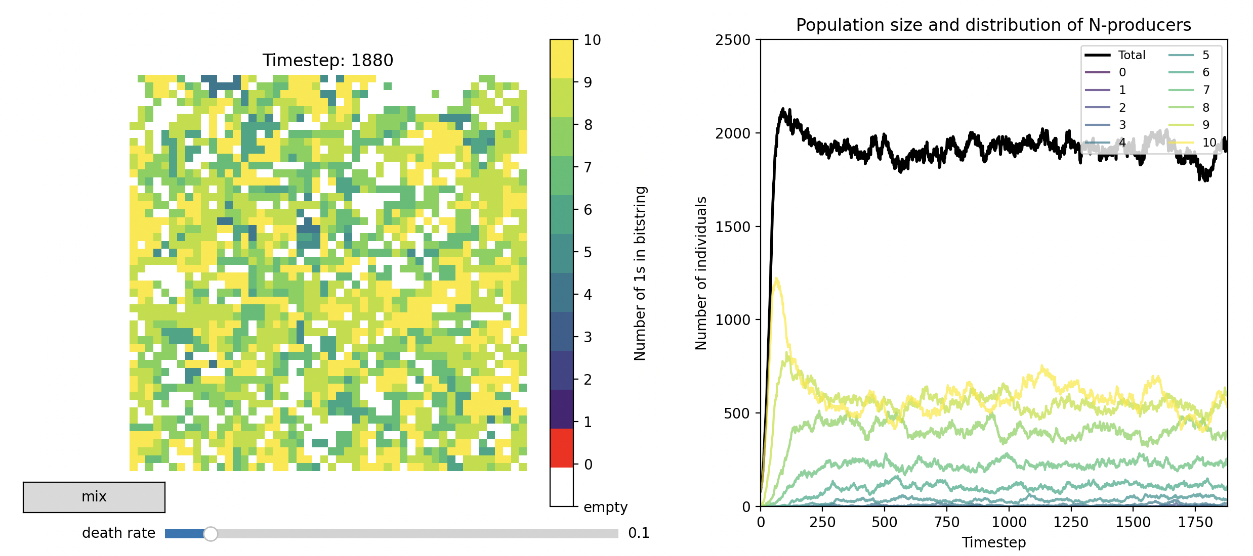
The model will have the following output: a grid that is coloured by the number of public goods produced (for consistency, let’s all use a ‘viridis’ scale), and a line graph that plots the total population sizes, as well as the population sizes of species producing 0 public goods, 1 public good, 2 public goods, etc. (see Figure 15.1)
Parameters to start out with
- Grid size: 50 x 50
- Initial population: produces all public goods (1111…1)
- Death rate: 0.1
- Cost (\(c\)): 0.05
- Bitstring 1 to 0 mutation (losing a gene): 0.01
- Bitstring 0 to 1 mutation (gaining a gene): 0.001
- Number of public goods (i.e. bitstring length): 10
- “No-event” size of roulette wheel: 1
Structure of code:
- Import libraries
- Set parameters
- Initialize grid
- Define simulation functions
- Set up interactive plot (and function)
- Run simulation (up until T=timesteps)
- Show final plot
Proposed experiments
Try investigating how the model behaves with different values of \(c\) (the cost of producing public goods). Can you explain what happens at \(c=0.0\)?
Try studying the effect of mixing the whole grid every timestep, such that neighbourhoods are constantly “randomised”. Look at the population size, as well as the distribution of different types. Can you explain the observations in biological terms?
Try studying what happens at different mutation rates.