14 What gets selected?
14.1 Genotypes, phenotypes, and evolutionary algorithms
During the lecture, we discussed the differences between the genotype (that which mutates) and the phenotype (that which is selected). Although you have likely already heard about these concepts, how can we study them in evolutionary models? During this practical, you will write your own evolutionary algorithms of increasing complexity, in order to learn about these topics. By the end of this practical, you should understand why the translation from genotype to phenotype (often referred to as the genotype-phenotype map) is such an important concept in evolutionary biology.
14.2 Simple model where fitness as a number
In the introduction of this course part on evolution, we have already looked at as simple “Moran process”:
- Start with a population of individuals, each with a fitness value.
- Select individuals based on their fitness to reproduce.
- Replace a random individual with this newly generate offspring.
- With a small probability, modify the ‘fitness’ value of the newborn.
And so on.
With a Moran process, competition between individuals is modeled in a very indirect (“implicit”) way. By always selecting fit individuals, and removing a random other, any individual in the populations could be replaced by another individual, which statistically is a fitter individual. One could thus say that “everyone is competing with everyone”. A different method is often applied in spatially structured models, as in this case only nearby individuals are competing. Then, we could sample who wins from an imaginary roulette wheel:
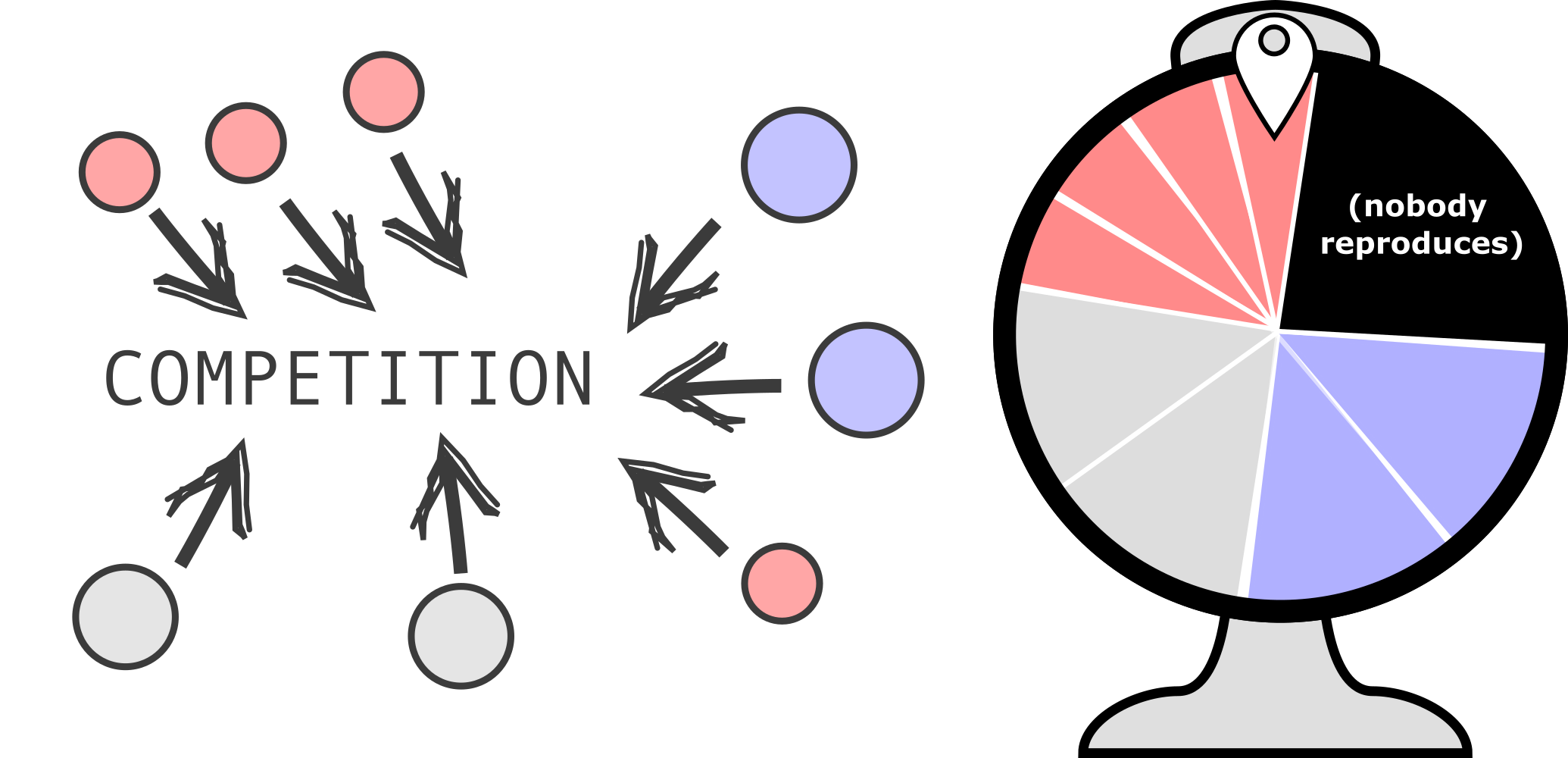
As can be seen, not all individual have the same size on the roulette wheel. That depicts differences in their growth rates, biomass, or other approximations of “fitness”. Also, the roulette wheel contains an area (shown in black) that shapes the chance that nobody reproduces. We will try and implement this rule to let individuals reproduce based on their fitness, but with only 10 competitors at a time. Let’s start with a code where individuals have a “fitness” value, but it not yet used for selection (see below). Read/test this code thoroughly before you move on to the next section.
import random
import math
import matplotlib.pyplot as plt

# Set the random number seed for reproducibility
random.seed(0)

plt.ion()  # Enable interactive plotting

# --- PARAMETERS ---
initial_fitness = 0.1            # Starting fitness for all individuals
population_size = 500             # Number of individuals (should be a square number for grid mode)
generations = 20000               # Number of generations to simulate
mutation_rate = 0.005            # Probability of mutation per reproduction event
sample_interval = 5               # How often to sample and plot data

# --- INITIALIZATION ---
# Create initial population: all individuals start with the same fitness
population = [initial_fitness for _ in range(population_size)]

# Lists to track average fitness and diversity over time
avg_fitness = []
diversity_over_time = []

# --- CORE FUNCTIONS ---

def mutate(fitness, rate=mutation_rate):
    """Mutate the fitness value with a given probability."""
    if random.random() < rate:
        # Fitness changes by a random value in [-0.1, 0.1], clipped to [0, 1]
        return min(1.0, max(0.0, fitness + random.uniform(-0.1, 0.1)))
    return fitness

def calculate_diversity(population):
    """NOT YET IMPLEMENTED! Calculate diversity as the standard deviation of fitness values."""
    return 0

# --- PLOTTING SETUP ---
fig, ax1 = plt.subplots(figsize=(12, 8))
ax1.set_xlabel("Generation")
ax1.set_ylabel("Average Fitness", color='tab:blue')
ax1.set_ylim(0, 1)
line1, = ax1.plot([], [], color='tab:blue', linewidth=2, label='Fitness')
ax1.tick_params(axis='y', labelcolor='tab:blue')

# Second y-axis for diversity
ax2 = ax1.twinx()
ax2.set_ylabel("Diversity", color='tab:green')
line2, = ax2.plot([], [], color='tab:green', linestyle=':', linewidth=2, label='Diversity')
ax2.tick_params(axis='y', labelcolor='tab:green')

fig.suptitle("Evolution Toward Fitness 1")
fig.tight_layout()
fig.legend(loc='upper right')
plt.grid(True)
plt.draw()

# --- EVOLUTION LOOP ---
found = False

for gen in range(generations):
    total_fit = sum(population)
    best = max(population)
    # Print when a perfect solution is found
    if best == 1 and not found:
        found = True
        print("Found perfect solution at generation", gen)

    # Sample and plot data at intervals
    if gen % sample_interval == 0:
        avg_fitness.append(total_fit / population_size)
        diversity_over_time.append(calculate_diversity(population))
        x_vals = [i * sample_interval for i in range(len(avg_fitness))]
        line1.set_data(x_vals, avg_fitness)
        line2.set_data(x_vals, diversity_over_time)
        ax1.relim(); ax1.autoscale_view()
        ax2.relim(); ax2.autoscale_view()
        fig.suptitle(f"Best Fitness: {best:.2f}", fontsize=14)
        plt.pause(0.01)


    # --- MORAN PROCESS ---
    # For each individual, perform a reproduction event
    for _ in range(100):  # 100 competition events per generation
        # Select 1 random individual for replication
        probs = [1 for fit in population] # All probability weights are equal (1.0)
        parent_idx = random.choices(range(len(population)), weights=probs)[0] # Grab one random individual based on an unweighted list...
        # Select individual to be replaced (uniform random)
        dead_idx = random.randrange(len(population))
        # Copy population for next generation
        new_pop = population.copy()
        # Offspring replaces the dead individual (with possible mutation)
        new_pop[dead_idx] = mutate(population[parent_idx])
        population = new_pop

input("\nSimulation complete. Press Enter to exit plot window...")
14.3 Making a roulette wheel with everyone in it
If you have read the code, you will see that we can pass a list of weights to the function random.choices, to determine who is most likely to be sampled. Currently, all the weights are set to 1:
probs = [1 for fit in population] # All probability weights are equal (1.0)
Exercise 14.1 (Running the roulette wheel with fitness values)
- Run the code with the current (all equal) weights. What happens?
- Modify this line of code to take the fitness values as the weight, rather than 1. (hint: this is a VERY small change in the code).
14.4 A roulette wheel of a subset of individuals
Instead of letting everyone reproduce, let us modify the code to only sample from a smaller list of ‘competitors’, and spin a virtual roulette wheel to determine who wins. There are many ways to implement this, but here’s how we will do it. We will sample \(N\) individuals from the population, and implement the following algorithm:
- Select a random subset of \(N\) individuals from the population.
- Take/compute the fitness of each selected individual.
- Add a reproduction-skip option with a fixed weight.
- Choose one individual or the skip option using weighted random selection.
- If an individual was chosen, mutate it and replace a random individual in the population.
Below, there’s a small snippet of code doing what is explained above1. The variable no_reproduction_chance is the fixed weight that nobody gets to reproduce:
  tournament_size = 10
  no_reproduction_chance = 1

  competitors = random.sample(population, tournament_size)
  # Make a list of their fitness values
  fitness_values = [fit for fit in competitors]
  total = sum(fitness_values)
  # Add a "no reproduction" dummy competitor with fitness = 0
  competitors_with_dummy = competitors + [None]
  probs = [f for f in fitness_values] + [no_reproduction_chance]
  winner = random.choices(competitors_with_dummy, weights=probs, k=1)[0]
  if winner is not None:
      # Mutate winner to produce offspring
      offspring = mutate(winner)
      remove_idx = random.randrange(len(population))
      population[remove_idx] = offspring
After you understand the roulette wheel algorithm, do the following exercise:
Exercise 14.2 (Questions about the roulette wheel - Algorithmic thinking)
- Let’s imagine a moment where the roulette wheel contains only 10 highly unfit individuals (e.g. all fitness values are 0.01). What is the chance that someone will reproduce? (you don’t have to calculate it, but give your reasoning)
- Answer the same question as in a., but now imagine that all 10 individuals have a fitness value of 1.
- Answer question b. and c. again, but now assume that
no_reproduction_chanceis equal to 0. - Describe what the
no_reproduction_chanceparameter does in biological terms. - Spatially structured populations are often placed on a grid. Describe how you could implement a roulette wheel to resolve local competition, e.g. when an empty grid point is competed for by the neighbours.
14.5 Diversity patterns
Modify the function calculate_diversity to calculate the diversity of the population as the standard deviation of the fitness values.
Exercise 14.3 (The dynamics of diversity - Biology)
- Use a low mutation rate and study the dynamics of diversity. Describe the pattern verbally.
14.6 Evolving a DNA sequence
A big problem with the previous model is there is no true distinction between genotype (that which mutates) and phenotype (that which is selected). Let us try and adapt the model to be more biologically meaningful, by making each individual represented by a DNA sequence. Copy the following code:
import random
import math
import matplotlib.pyplot as plt
from collections import Counter

# set the random number seed
random.seed(0)

plt.ion()  # Enable interactive mode

# Parameters
alphabet = "ATCG"
target_sequence = "GATGCGCGCTGGATTAAC"  # Example target sequence
dna_length = len(target_sequence)
target_length = len(target_sequence)

# Simulation settings
population_size = 500  # must be a square number for grid mode
generations = 20000
mutation_rate = 0.001
sample_interval = 5
sample_size = population_size
no_reproduction_chance = 0.1

# Core functions
def fitness(dna):
    return 1 - sum(a != b for a, b in zip(dna, target_sequence)) / target_length

def mutate(dna, rate=mutation_rate):
    return ''.join(
        random.choice([b for b in alphabet if b != base]) if random.random() < rate else base
        for base in dna
    )

def count_beneficial_mutations(dna):
    f0 = fitness(dna)
    count = 0
    for i in range(len(dna)):
        for b in alphabet:
            if b != dna[i]:
                mutant = dna[:i] + b + dna[i+1:]
                if fitness(mutant) > f0:
                    count += 1
    return count

def diversity(pop):
    counts = {}
    for ind in pop:
        counts[ind] = counts.get(ind, 0) + 1
    total = len(pop)
    return -sum((c/total) * math.log(c/total + 1e-9) for c in counts.values()) if total > 0 else 0

# Initialize population
initial_sequence = "GATAGCGAAGTTTAGCCG" # far from target (only first 3 are correct)
population = [initial_sequence for _ in range(population_size)]

avg_fitness = []
avg_beneficial = []
diversity_over_time = []
best_individuals = []

def get_neighbors(i, j):
    return [(x % side, y % side)
            for x in range(i-1, i+2)
            for y in range(j-1, j+2)]

# Initialize interactive plot
fig, ax1 = plt.subplots(figsize=(12, 8))
ax1.set_xlabel("Generation")
ax1.set_ylabel("Average Fitness", color='tab:blue')
ax1.set_ylim(0, 1)
line1, = ax1.plot([], [], color='tab:blue', linewidth=2, label='Fitness')
ax1.tick_params(axis='y', labelcolor='tab:blue')

ax2 = ax1.twinx()
ax2.set_ylabel("Beneficial Mutations / Diversity", color='tab:purple')
line2, = ax2.plot([], [], color='tab:purple', linestyle='--', linewidth=2, label='Beneficial Mutations')
line3, = ax2.plot([], [], color='tab:green', linestyle=':', linewidth=2, label='Diversity')
ax2.tick_params(axis='y', labelcolor='tab:purple')
fig.suptitle("Evolution Toward Target Sequence")
fig.tight_layout()
ax2.set_ylim(0, 20)
fig.legend(loc='upper right')
plt.grid(True)
plt.draw()

best_seq = ""
best_score = -1
found = False

# Evolution loop
for gen in range(generations):
    fitnesses = [fitness(ind) for ind in population]
    total_fit = sum(fitnesses)
    best = max(fitnesses)
    if(best == 1 and not found):
        found = True
        print("Found perfect solution at generation", gen)

    if gen % sample_interval == 0:
        sample = random.sample(population, sample_size)
        avg_beneficial.append(sum(count_beneficial_mutations(ind) for ind in sample) / sample_size)
        diversity_over_time.append(diversity(population))

        # Update plot data
        line1.set_data(range(len(avg_fitness)+1), avg_fitness + [sum(fitnesses)/population_size])
        line2.set_data(range(len(avg_beneficial)), avg_beneficial)
        line3.set_data(range(len(diversity_over_time)), diversity_over_time)
        ax1.relim(); ax1.autoscale_view()
        ax2.relim(); ax2.autoscale_view()
        best = max(population, key=fitness)
        fig.suptitle(f"Best: {best} (target: {target_sequence})", fontsize=14)
        plt.pause(0.01)

    else:
        avg_beneficial.append(avg_beneficial[-1])
        diversity_over_time.append(diversity_over_time[-1])

    # Tournament selection (as in evolving_fitness_final.py)
    new_pop = []
    tournament_size = 10  # can be adjusted

    for _ in range(population_size):
        # Select tournament_size individuals randomly
        competitors = random.sample(population, tournament_size)
        # Pick the one with highest fitness
        fitness_values = [fitness(ind) for ind in competitors]
        total = sum(fitness_values)

        probs = [f / total for f in fitness_values]
        winner = random.choices(competitors, weights=probs, k=1)[0]
        # Mutate winner to produce offspring
        offspring = mutate(winner)
        new_pop.append(offspring)

    population = new_pop

    avg_fitness.append(sum(fitness(ind) for ind in population) / population_size)
    if gen % 250 == 0:
        best = max(population, key=fitness)
        best_individuals.append((gen, best))

input("\nSimulation complete. Press Enter to exit plot window...")
Answer the following questions using the options available in the model:
Exercise 14.4 (Evolving DNA - Biology / abstract thinking)
- Run the code. What does the new (dashed blue) line represent? Do you understand how it changes over time?
The program reports after how many generations it manages to find the target sequence. With default settings this can take a long time… (default: 429 generations)
- Modify the mutation rate to see how it affects the time to find the target sequence. Try different mutation rates between 0.0001 and 0.1. Keep track of both how long (number of generations) it takes to find the target, and how fit the population is once the target is found. What do you observe?
- Diversity is no longer calculated as the standard deviation in fitness, but as the Shannon diversity of all present sequences (although it is not super complex, you do not need to fully understand this function). Because of this, the exact number (quantities) cannot be compared to our earlier model. Do you see a qualitative differences?
- Study how fitness is calculated in this model. Is there a distinction between genotype en phenotype? Why/why not?
14.7 Evolving a protein sequence
Next we will extend the simulation a little more. The individual genotypes will still be represented as a DNA sequence, but before evaluating fitness this will be translated into a protein sequence. To do so, the code first defines the codon table (which we of course all know by heart =)), and then translates the DNA sequence into a protein sequence. The protein sequence is then used to calculate the fitness of the individual, which is based on how well the protein sequence matches a target protein sequence. The code is as follows:
import random
import math
import matplotlib.pyplot as plt
from collections import Counter

# set the random number seed
random.seed(0)

plt.ion()  # Enable interactive mode

# Codon table
codon_table = {
    'TTT': 'F', 'TTC': 'F', 'TTA': 'L', 'TTG': 'L', 'CTT': 'L', 'CTC': 'L', 'CTA': 'L', 'CTG': 'L',
    'ATT': 'I', 'ATC': 'I', 'ATA': 'I', 'ATG': 'M',
    'GTT': 'V', 'GTC': 'V', 'GTA': 'V', 'GTG': 'V',
    'TCT': 'S', 'TCC': 'S', 'TCA': 'S', 'TCG': 'S', 'AGT': 'S', 'AGC': 'S',
    'CCT': 'P', 'CCC': 'P', 'CCA': 'P', 'CCG': 'P',
    'ACT': 'T', 'ACC': 'T', 'ACA': 'T', 'ACG': 'T',
    'GCT': 'A', 'GCC': 'A', 'GCA': 'A', 'GCG': 'A',
    'TAT': 'Y', 'TAC': 'Y', 'CAT': 'H', 'CAC': 'H',
    'CAA': 'Q', 'CAG': 'Q', 'AAT': 'N', 'AAC': 'N',
    'AAA': 'K', 'AAG': 'K', 'GAT': 'D', 'GAC': 'D',
    'GAA': 'E', 'GAG': 'E', 'TGT': 'C', 'TGC': 'C',
    'TGG': 'W', 'CGT': 'R', 'CGC': 'R', 'CGA': 'R', 'CGG': 'R', 'AGA': 'R', 'AGG': 'R',
    'GGT': 'G', 'GGC': 'G', 'GGA': 'G', 'GGG': 'G',
    'TAA': '*', 'TAG': '*', 'TGA': '*'
}

# Parameters
alphabet = "ATCG"
target_protein = "DARWIN"
dna_length = len(target_protein)*3
target_length = len(target_protein)

# Simulation settings
population_size = 625  # must be a square number for grid mode
generations = 20000
mutation_rate = 0.0005
sample_interval = 5
sample_size = population_size
no_reproduction_chance = 0.01

# Core functions
def translate(dna):
    return ''.join(codon_table.get(dna[i:i+3], '?') for i in range(0, len(dna), 3))

def fitness(dna):
    protein = translate(dna)
    return 1 - sum(a != b for a, b in zip(protein, target_protein)) / target_length

def mutate(dna, rate=mutation_rate):
    return ''.join(
        random.choice([b for b in alphabet if b != base]) if random.random() < rate else base
        for base in dna
    )

def count_beneficial_mutations(dna):
    f0 = fitness(dna)
    count = 0
    for i in range(len(dna)):
        for b in alphabet:
            if b != dna[i]:
                mutant = dna[:i] + b + dna[i+1:]
                if fitness(mutant) > f0:
                    count += 1
    return count

def diversity(pop):
    counts = Counter(pop)
    total = len(pop)
    return -sum((c/total) * math.log(c/total + 1e-9) for c in counts.values()) if total > 0 else 0

# Initialize population
initial_sequence = ''.join(random.choice(alphabet) for _ in range(dna_length))
population = [initial_sequence for _ in range(population_size)]

avg_fitness = []
avg_beneficial = []
diversity_over_time = []
best_individuals = []

# Grid setup
side = int(math.sqrt(population_size))
assert side * side == population_size, "Population size must be a square number for grid mode"

def get_neighbors(i, j):
    return [(x % side, y % side)
            for x in range(i-1, i+2)
            for y in range(j-1, j+2)]

# Initialize interactive plot
fig, ax1 = plt.subplots(figsize=(12, 8))
ax1.set_xlabel("Generation")
ax1.set_ylabel("Average Fitness", color='tab:blue')
ax1.set_ylim(0, 1)
line0, = ax1.plot([], [], color='black', linewidth=1, label='Max fitness')
line1, = ax1.plot([], [], color='tab:blue', linewidth=2, label='Fitness')
ax1.tick_params(axis='y', labelcolor='tab:blue')

ax2 = ax1.twinx()
ax2.set_ylabel("Beneficial Mutations / Diversity", color='tab:purple')
line2, = ax2.plot([], [], color='tab:purple', linestyle='--', linewidth=2, label='Beneficial Mutations')
line3, = ax2.plot([], [], color='tab:green', linestyle=':', linewidth=2, label='Diversity')
ax2.tick_params(axis='y', labelcolor='tab:purple')
fig.suptitle("Evolution Toward " + str(target_protein))
fig.tight_layout()
ax2.set_ylim(0, 5)
fig.legend(loc='upper right')
plt.grid(True)
plt.draw()

best_seq = ""
best_score = -1
best_fitnesses = []
found = False

# Evolution loop
for gen in range(generations):
    fitnesses = [fitness(ind) for ind in population]
    total_fit = sum(fitnesses)
    best = max(fitnesses)
    best_fitnesses.append(best)
    if(best == 1 and not found):
        found = True
        print("Found perfect solution at generation", gen)

    if gen % sample_interval == 0:
        sample = random.sample(population, sample_size)
        avg_beneficial.append(sum(count_beneficial_mutations(ind) for ind in sample) / sample_size)
        diversity_over_time.append(diversity(population))

        # Update plot data
        line0.set_data(range(len(avg_fitness)+1), best_fitnesses)
        line1.set_data(range(len(avg_fitness)+1), avg_fitness + [sum(fitnesses)/population_size])
        line2.set_data(range(len(avg_beneficial)), avg_beneficial)
        line3.set_data(range(len(diversity_over_time)), diversity_over_time)
        ax1.relim(); ax1.autoscale_view()
        ax2.relim(); ax2.autoscale_view()
        best = max(population, key=fitness)
        fig.suptitle(f"Best: {translate(best)} (target: {target_protein})", fontsize=14)
        plt.pause(0.01)

    else:
        avg_beneficial.append(avg_beneficial[-1])
        diversity_over_time.append(diversity_over_time[-1])

    new_pop = []
    tournament_size = 10  # can be adjusted

    for _ in range(population_size):
        # Select tournament_size individuals randomly
        competitors = random.sample(population, tournament_size)
        # Pick the one with highest fitness
        fitness_values = [fitness(ind) for ind in competitors]
        total = sum(fitness_values)

        probs = [f / total for f in fitness_values]
        winner = random.choices(competitors, weights=probs, k=1)[0]
        # Mutate winner to produce offspring
        offspring = mutate(winner)
        new_pop.append(offspring)

    population = new_pop


    avg_fitness.append(sum(fitness(ind) for ind in population) / population_size)
    if gen % 250 == 0:
        best = max(population, key=fitness)
        best_individuals.append((gen, translate(best)))

input("\nSimulation complete. Press Enter to exit plot window...")
Answer the following question about the model:
Exercise 14.5 (Evolving protein sequences - Biology / abstract thinking)
- Another line was added to the model. What new information can you obtain from analysing this line?
- Study carefully how the other lines (also present in previous models) change over time. What do you observe? Try and capture what you see into words.
- In biology, multiple genotypes can translate to the same phenotype (this is called a many-to-one genotype-phenotype map), or alternatively, one genotype can produce multiple phenotype (this is called phenotypic plasticity, or a one-to-many genotype-phenotype map). Which genotype-phenotype (GP) mapping applies to this model? Why?
- Bonus question for motivated students modify the code to include a second target protein sequence, and alternate between the two targets. If you see something interesting, please share it with the class!
- Bonus question for motivated students modify the code to include spatial structure in the population (e.g. proteins on a grid only competing with nearby proteins).
Note that this is from the full code, so this code does not work stand-alone↩︎